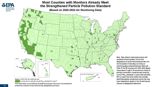
• On February 7, 2024, the U.S. Environmental Protection Agency (EPA) announced a final
  rule to strengthen the nation’s National Ambient Air Quality Standards (NAAQS) for fine particulate matter (PM2.5). EPA has set the level of the primary (health-based) annual PM2.5 standard at 9.0 micrograms per cubic meter (ug/m3). The Agency has provided a map based on 2020-2022 air quality data illustrating the counties that currently meet and those that currently violate the lowered annual PM2.5 standard. Official nonattainment designations using the revised annual PM2.5 standard will occur sometime in the future.

Additional information can be found by clicking here.

• In January 2023, the EPA indicated that as a result of the CASAC's comments and recommendations on the EPA's ozone 2020 Integrated Science Assessment document, the Agency was going to prepare a revision of its first draft of its "Policy Assessment for the Reconsideration of the Ozone National Ambient Air Quality Standards" document. In early March 2023, the EPA published its second draft policy assessment document. The draft document was prepared as a part of the reconsideration of the 2020 final decision on the national ambient air quality standards (NAAQS) for ozone (O3). Dr. Lefohn's comments on the first draft document were submitted on May 30, 2022 to the official Docket and are available by clicking here. Dr. Lefohn's comments on the second draft document were submitted on April 10, 2023 to the official Docket and are available by clicking here. In the second draft of the Policy Assessment document, the EPA noted that it anticipated that the reconsideration of the ozone standards could not be completed any more expeditiously than by the end of 2024. EPA indicated in its second draft that the Agency planned to submit a draft of the Administrator's decision on the ozone standards by April 2024. CASAC completed its ozone assignment by reviewing the second draft of the Policy Assessment document and recommended to the EPA Administrator in a letter on June 9, 2023 that the primary and secondary ozone standards be changed. The current ozone primary standard is 70 ppb and CASAC recommended that the Administrator consider for the human health ozone standard a range of 55 to 60 ppb. The current ozone secondary standard is the same as the primary standard and CASAC recommended to the Administrator that the form of the secondary standard should be changed to the cumulative W126 exposure metric, an index recommended by several previous CASAC ozone panels, as well as at times by the EPA, to protect vegetation. CASAC recommended that the Administrator consider that the level of the W126 metric be in the range of 7 to 9 ppm-hrs. The June 9, 2023 CASAC letter to the EPA Administrator can be read by clicking here. Upon considering the CASAC recommendations for the human health and vegetation ozone standards, in August 2023 the EPA decided to initiate a new review of the ozone NAAQS, which meant that the entire ozone rulemaking process would be initiated once again. In its August 18, 2023 letter to the Chair of CASAC, the EPA Administrator states

I remain committed to upholding the integrity and rigor of the NAAQS review process and to addressing the issues that CASAC has raised. Given the scope of those issues and the EPA’s obligation under the Clean Air Act to conduct periodic five-year reviews of the air quality criteria and the standards, I have decided that the best path forward is to initiate a new statutory review of the ozone NAAQS and the underlying air quality criteria and to wrap the EPA’s reconsideration process of the 2020 ozone NAAQS decision into that review. This approach would facilitate additional work to address CASAC’s advice, as well as consideration of newer studies and updated analyses, in the context of a full and systematic review of the air quality criteria and standards, with the opportunities for CASAC advice and public engagement that such a process involves. I have instructed my staff to immediately announce a new review of the ozone NAAQS, as well as the underlying air-quality criteria, and to complete this review as expeditiously as possible, while also upholding the scientific integrity and rigor of the NAAQS review process and providing opportunities for public input and engagement.

The August 18, 2023 letter can be read by clicking here. According to the legal requirement that the standards have to be reviewed every 5 years, the ozone review process will have to be completed by December 2025, which is 5 years following the EPA's 2020 decision. Previous attempts to develop written materials for public review, receive CASAC's comments on the written materials, and produce a final decision by the EPA Administrator have usually taken more than the required 5 years with the result that litigation has often been initiated.

In initiating its new ozone review, the EPA convened a public science and policy workshop on May 13 through May 16, 2024 to gather input from the scientific community and the public. Following the workshop, EPA developed a workshop proceedings document that was made available on September 30, 2024 on the EPA website. In addition, a three-volume Integrated Review Plan (IRP) for the review of the ozone NAAQS will be developed. Volume 1 will provide background on the ozone NAAQS. Volume 2 is the planning document for the review and the ISA, and will outline the schedule, process, and approaches for evaluating the relevant scientific information and addressing the key policy-relevant issues to be considered in the review. Volume 3 is the planning document for technical air quality, exposure, and risk analyses. For more information about EPA's Integrated Science Assessment activities, please click here.

• The EPA told the U.S. Court of Appeals for the D.C. Circuit in a court filing in late October 2021 that it would initiate a rulemaking process to reassess by the end of 2023 the Agency's December 2020 decision to retain the 2015 ozone human health and vegetation standards. https://bit.ly/3HDC2ov

• The DC Court of Appeals on August 23, 2019 rendered its decision on the EPA’s 2015 ozone (smog) standards. The Court remanded back to the EPA for reconsideration the ozone standard to protect vegetation. The W126 metric, created by Dr. A.S. Lefohn, which the current CASAC recommended to protect vegetation, is involved in this decision. For more information, please read the entire decision by the Court.

• The EPA Administrator made the Agency's final ozone rulemaking decision on its previous review on December 23, 2020. Both the human health and vegetation ozone standards remained at the levels established in 2015. The EPA's decision on the ozone standards can be reviewed here. When the EPA reconsidered the December 2020 decision on both the human health and vegetation ozone standards, additional focus was on the use of the current 8-h ozone standard as a means to control W126 exposure values for the protection of vegetation. In his comments on the "Policy Assessment for the Reconsideration of the Ozone National Ambient Air Quality Standards, External Review Draft document, Dr. Lefohn focused some of his comments on the EPA's use of the current primary 8-h standard to control for W126 exposures that affect vegetation. His May 30, 2022 comments to the Docket can be viewed here. In his most recent comments, which focused on the second draft of the Policy Assessment document, Dr. Lefohn again focused some of his comments on the use of the current primary 8-h standard to control for W126 exposures that affect vegetation. His comments can be viewed here.

On October 1, 2020, Dr. Lefohn, President of A.S.L. & Associates, LLC, responded to EPA's request for comments on the draft ozone rulemaking proposal. His 222 page document, filed in the official Docket, can be downloaded here. In December 2019, his comments on the drafts of the EPA's Integrated Science Assessment for Ozone (ISA) and Policy Assessment (PA) documents were filed in the U.S. government's official Docket. Dr. Lefohn's comments on the Integrated Science Assessment for Ozone (ISA) report can be downloaded here. His comments on the first draft of the Policy Assessment (PA) document can be downloaded here. His April 10, 2023 comments on the second draft of the Policy Assessment document, which contain 302 pages, can be read here. Some of the points made in the submissions were

• There are two fundamental principles important in the ozone rulemaking activity.

• Fundamental Principle One: Higher Hourly Average Ozone Concentrations Should be Weighted More than Middle and Lower Values when Assessing Human Health and Environmental Effects. The use of long-term average concentrations is not supported by human health and vegetation laboratory experiments. Based on ozone laboratory experiments, Haber's Rule (i.e., concentration multiplied by time) is not appropriate.

• Fundamental Principle Two: Daily Maximum Hourly Averaged Ozone Concentrations Will Remain Well above 0 Parts per Billion (ppb) Even if all Anthropogenic Emissions Were Eliminated Worldwide. In other words, there are natural sources of ozone that contribute substantially to surface ozone concentrations that are measured daily around the world.

• As a result of emission reductions, at many locations the highest ozone concentrations are reduced and the lowest concentrations are increased due to the reduction of NO scavenging.

• Annual average or median concentrations increase as emissions are reduced at some monitoring sites in the US. This is a result of the reduction of NO scavenging on the lower concentrations.

• In 2015, EPA noted in its ozone rulemaking process that both acute and chronic ozone health effects could be reduced by reducing the higher hourly average concentrations. This is an important statement by the Agency because it indicates that ozone exposure metrics, used in models for estimating long-term risk to humans, should be focused on the reduction of the higher ozone values rather than attempting to reduce the entire distribution of hourly average concentrations. The use of ozone exposure metrics, based on annual average concentrations which increase at many sites because of the reduction of NO scavenging associated with emission reductions, could result in less than accurate human health ozone risk estimates.

• The body of evidence calls into question the adequacy of the protection for vegetation provided by the current secondary ozone standard. An alternative form and level is required to adequately protect vegetation.

• The Working Group I contribution to the IPCC's Sixth Assessment Report, AR6 Climate Change 2021: The Physical Science Basis, addresses the latest physical understanding of the climate system and climate change. The report is an interesting read. The report can be downloaded at https://www.ipcc.ch/report/ar6/wg1/.

• In a recent published article, Go slow to go fast: A plea for sustained scientific rigor in air pollution research during the COVID-19 pandemic, the authors (Heederik, Smit, and Vermeulen), all associated with the Division of Environmental Epidemiology, Institute for Risk Assessment Sciences, Utrecht University, Utrecht, The Netherlands, noted that over a ten-day period, three papers involving original research associating COVID-19 mortality and air pollution were published. These publications attracted considerable attention from international news outlets and on social media. According to the authors, all three ecological studies relied on aggregate data, which can suffer from the well-known problem of ecological fallacy, where a misjudgment in interpretation occurs as inferences about individuals are reasoned from the group to which the individual belongs. The authors believe that this is a major issue, mostly ignored in these studies resides in the complexity of a potential association between air pollution and COVID-19 morbidity and mortality. The authors' article was published in the European Respiratory Journal. The Journal is the flagship journal of the European Respiratory Society. The entire article can be downloaded at https://bit.ly/3hHRxO6.

• Design values published by the EPA provide an opportunity to quantitatively evaluate for the period 2015-2017 the status of ozone (smog) exposures in the national parks in the United States. Ozone data from 43 monitors in the US national park system were evaluated for potential human health risk. Sixty-one percent of the monitoring sites in the park system received a grade of either "A" or "B", 12% received a grade of "C", and 28% received a grade of either "D" or "F". More information available at https://bit.ly/2MfFuM4.

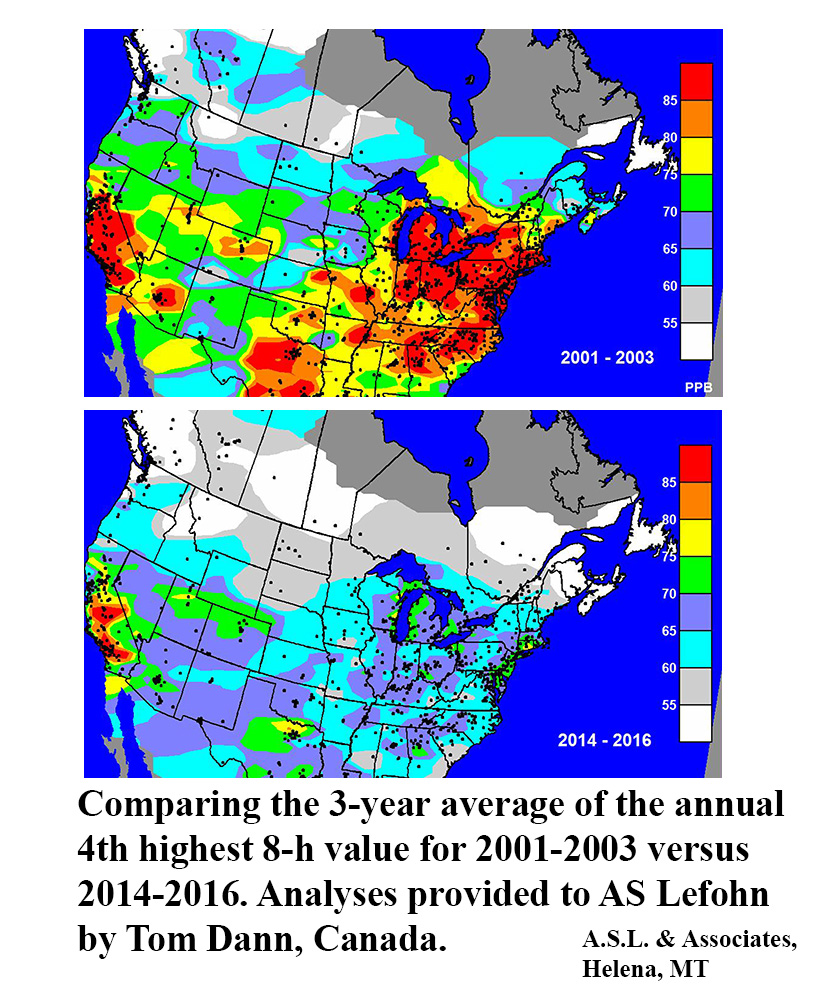
• Over the years in the United States, we made considerable progress in reducing ozone (i.e., smog) exposures. The 3-year average of the annual 4th highest daily 8-h concentration is the form of the US ozone standard to protect human health and welfare (i.e., vegetation). In 2015, the US EPA lowered the standard to 70 parts-per-billion (ppb). More information available at https://bit.ly/2sLxbMU.

• The use of different air quality markers (metrics) for surface ozone calculated from the same time series can result in different trend patterns. This outcome is important to researchers, as well as policymakers and regulators, who use exposure metrics to assess how changes in ozone levels affect human health, vegetation, and climate.

That's one conclusion from a metrics assessment based on the Tropospheric Ozone Assessment Report or TOAR, an effort by the International Global Atmospheric Chemistry Project to create the world's largest database of surface ozone observations from all available ozone monitoring stations around the globe. The TOAR paper, Global surface ozone metrics identified for climate change, human health, and crop/ecosystem research, was published in the journal Elementa: Science of the Anthropocene. The list of metrics used in the TOAR program can be downloaded here. The paper is available at the Elementa website at: https://www.elementascience.org/article/10.1525/elementa.279/

The 24 international researchers who worked on the paper anticipate that their effort will provide scientists, regulators, and policymakers with better insight about spatial and temporal variation that relate to climate change, human health, and crop/ecosystem around the world.

The paper provides the following:

• A description of 25 metrics, which are used for assessing spatial and temporal trends by environmental agencies and researchers around the world (4 for model-measurement comparison, 5 for characterization of ozone in the free troposphere, 11 for human health impacts, and 5 for vegetation impacts).

• The scientific rationale for the selection of each of the 25 metrics.

• A detailed description of the statistical methods based on stringent scientific principles used in the Tropospheric Ozone Assessment Report (TOAR) program.

• A comparison of the trend behavior for each of the ozone impact metrics when using the same surface ozone concentration time series.

Key components of the Tropospheric Ozone Assessment Report (TOAR) (http://www.igacproject.org/activities/TOAR) are the use of metrics that are biologically defensible, as well as the use of statistical methods that adhere to stringent scientific principles. This paper provides the background for the selection of the metrics and the statistical methods used in the international TOAR program.

• Background ozone is an important part of the challenge to attaining the 0.070 ppm ozone standard. Although the EPA is continuing the ozone area designation process, the Agency is still concerned about the effect that background has on attainment of the 2015 ozone standard. Specifically, the key reasons that the EPA proposed a delay in 2017 to implementing the new ozone standard were

• Fully understanding the role of background ozone levels;
• Appropriately accounting for international transport; and
• Timely consideration of exceptional events demonstrations.

There is much controversy on what the range of background ozone is in the United States. Our research is indicating that frequent occurrences greater than or equal to 50 ppb that occur at both high- and low-elevation monitoring sites across the US are influenced by transport from the stratosphere to the lower troposphere. The enhanced ozone concentrations that appear to be related to stratospheric transport occur during the springtime and sometimes during the summertime. In addition, long-range transport of Eurasian biomass burning, as well as wildfires in the US, contribute to background ozone concentrations. Estimating the range of background ozone properly is important because the range of background concentrations is used in the EPA's risk assessment for human health and vegetation, as well as assessing the amount of emission reductions required to attain a specific ozone level (i.e., standard). If the actual background level of ozone is higher than EPA estimates with models, then the Agency may overestimate human health, as well as vegetation risks and present inaccurate information to the public and policymakers. Our published material on background ozone can be found here. Our current research continues to address how to integrate background ozone with the attainment process.

• Since A.S.L. & Associates' founder, Dr. Allen Lefohn, participated like others in the first Earth Day on April 22, 1970, we have seen much progress in controlling environmental pollution and improving the Nation's health and welfare (i.e., vegetation). For example, the US EPA began to regulate ozone with the promulgation of a ground-level National Ambient Air Quality Standard (NAAQS) in 1971, with subsequent revisions in 1979, 1997, 2008, and 2015. Following promulgation of the 1997 ozone standard, the US EPA issued a NOx State Implementation Plan (SIP) Call, which reduced regional summertime NOx emissions from power plants and other large stationary sources by 57% in 22 Eastern US states. In addition, the US EPA established national rules that substantially reduced NOx and VOC emissions from on-road mobile sources by 53% and 77% between 1990 and 2014, respectively. Overall, NOx and VOC have decreased in the US by 52% and 39% from all sources since 1990.

• Changes in the magnitude of national and regional emissions, as well as any long-term changes in international emissions, climate, and inter-annual meteorological variability, can drive shifts in the distributions of hourly surface ozone (O3) concentrations. Changes in the distributions of hourly average O3 concentrations can result in changes in the magnitude of exposure metrics used for assessing human health and vegetation effects. Surprisingly, trend patterns in O3 exposure metrics may be in a similar direction as emissions change (e.g., metrics increase as emissions increase) or trend patterns of metrics may not be in a similar direction as emissions change (e.g., metrics increase as emissions decrease) (Lefohn et al., 2017; Lefohn et al., 2018 - see publications list). Besides the work by Lefohn et al. (2017, 2018), other researchers have reported this observation in the literature. This is a very important observation because if a biologically irrelevant O3 metric is selected for assessing trends, an incorrect conclusion may be drawn concerning the relationship between emissions reductions and the protection of the public's health and welfare. Over the past 20-30 years, substantial changes in O3 concentrations have been observed at many sites across the world, likely driven by a combination of the large emissions changes and potentially by shifts in various meteorological conditions. The paper by Lefohn et al. (2017) investigated the relationship between exposure metrics, hourly O3 concentration distributions, and emission changes. To achieve this, we analyzed the response of 14 human health and vegetation O3 metrics to long-term changes in the hourly O3 concentration distribution, as measured at 481 monitoring sites in the EU, US, and China. The study provided insight into the utility of using specific exposure metrics for assessing emission control strategies. One important aspect of the study was that trends in mean or median concentrations did not appear to be well associated with some of the exposure metrics applicable for assessing human health or vegetation effects. Additional insights concerning the relationships between emissions reductions, hourly average concentration distributions, and human health and vegetation exposure metrics are discussed in Lefohn et al. (2017) and Lefohn et al. (2018) (please see publications list).

• In October 2015, the EPA announced that both the human health and vegetation ozone standards were 70 ppb. Prior to that, on November 26, 2014, the EPA Administrator proposed an ozone human health (primary) standard in the range of 65 to 70 ppb and indicated that she would take comment on a standard as low as 60 ppb. The EPA Administrator noted that she placed the greatest weight on controlled human exposure studies, citing significant uncertainties with epidemiologic studies. Reasons for placing less weight on epidemiologic-based risk estimates were key uncertainties about (1) which co-pollutants were responsible for health effects observed, (2) the heterogeneity in effect estimates between locations, (3) the potential for exposure measurement errors, and (4) uncertainty in the interpretation of the shape of concentration-response functions for ozone concentrations in the lower portions of ambient distributions. The health standard is mainly based on the controlled human exposure study of Schelegle et al. (2009) that reported clinical effects at 72 ppb. Dr. Milan Hazucha of UNC Chapel Hill and Dr. Lefohn, A.S.L. & Associates) designed the ozone hourly exposure regimes used in the Schelegle et al. (2009) study. To the 72 ppb threshold of effects resulting from the Schelegle et al. (2009) study, the Administrator applied a Margin of Safety that helped her establish the ozone health standard below the 72 ppb level. Although the CASAC recommended a separate exposure metric for the secondary standard (the W126 vegetation metric), the EPA adopted the 8-hour standard of 0.070 ppm to protect vegetation. The Agency believed that the 3-month, 12-h W126 exposure index used for assessing vegetation effects could be controlled to a level of 17 ppm-h or less by using the 8-hour standard. Industry and environmental organizations are back in court contesting the decision of the 8-hour ozone standard set at the 0.070 ppm level. On August 23, 2019, the D.C. Court of Appeals rendered its decision on the various challenges to the Environmental Protection Agency's 2015 revisions to the primary and secondary national ambient air quality standards for ozone. The Court denied the petitions, except with respect to the secondary ozone standard, which it remanded for reconsideration, and grandfathering provision, which the Court vacated.The Court of Appeal's decision makes interesting reading and is available by clicking here. Although the EPA attempted to address in December 2020 several of the Court's concerns about the Agency's 2015 decision on the ozone vegetation standard, there still remain deficiencies in the Agency's rationale. Perhaps in the reconsideration process for the 2015 ozone standards, these deficiences will be addressed during the 2022-2023 deliberations.

Some historical perspective is important in understanding the background concerning the events that led to the EPA's Administrator's decision on revising the 8-hour ozone standard in October 2015. On March 12, 2008, the EPA Administrator announced a decision on the human health and vegetation ozone standards. At that time, EPA revised the 8-hour "primary" ozone standard, designed to protect public health, to a level of 0.075 parts per million (ppm). The previous standard, set in 1997, was 0.08 ppm. EPA decided not to adopt the cumulative exposure index as the vegetation standard (i.e., secondary ozone standard). Although the EPA Administrator recommended the W126 index as the secondary ozone standard, based on advice from the White House (Washington Post, April 8, 2008; Page D02), the EPA Administrator made the secondary ozone standard the same as the primary 8-hour average standard (0.075 ppm). On May 27, 2008, health and environmental organizations filed a lawsuit arguing that the EPA failed to protect public health and the environment when it issued in March 2008 new ozone standards. On March 10, 2009, the US EPA requested that the Court vacate the existing briefing schedule and hold the consolidated cases in abeyance. EPA requested the extension to allow time for appropriate EPA officials that were appointed by the new Administration to review the Ozone NAAQS Rule to determine whether the standards established in the Ozone NAAQS Rule should be maintained, modified, or otherwise reconsidered. After an extensive review process, the Obama Administration decided to not revise the 0.075 ppm standard that was set during the Bush Administration. The reason provided was that the EPA would soon begin a new review cycle of the science associated with surface ozone and recommend whether the 0.075 ppm standard needed to be revised.

• For several years, A.S.L. & Associates has had an on-going effort to better understand the range and frequency of occurrence of background ozone levels that may not be affected by emission reduction strategies. In a paper published in May 2001, the research team consisting of Allen Lefohn, Samuel Oltmans, Tom Dann, and Hanwant Singh discussed that background ozone levels were higher and that the natural short-term variability was more frequent and greater than previously believed. In our 2001 paper, we concluded that hourly levels greater than or equal to 50 ppb occur more frequently as a result from natural sources than previously believed. In 2006, the US EPA defined Policy-Relevant Background (PRB) for ozone as those concentrations that would occur in the United States in the absence of anthropogenic emissions in continental North America (i.e., the United States, Canada, and Mexico). PRB concentrations (renamed by the EPA as North American Background (NAB)) include contributions from (1) natural sources everywhere in the world and (2) anthropogenic sources outside the United States, Canada, and Mexico. In 2008, we published results, using empirical data, confirming that at some locations in the US, background ozone concentrations were greater than or equal to 50 ppb. In September 2009, the National Research Council released the report, Global Sources of Local Pollution. In the report, the Committee stated that modeling and analysis supports the finding that background was 20-40 ppb for the United States. Unfortunately, the NRC conclusion did not agree with the peer-review literature using empirical data that showed that hourly averaged background ozone concentrations at times were greater than or equal to 50 ppb. Although spatially low-resolution models were exercised at the time that indicated that conclusions reached by Lefohn et al. (2001) were incorrect, our current research and the results published by other research groups support the conclusions reached by Lefohn et al. (2001) that backgrund ozone concentrations are greater than or equal to 50 ppb at both high- and low-elevation monitoring sites. An Internet-based slide presentation is available for purposes of previewing our paper. Also please be sure to check out the answer to our quiz that identifies the month in which the highest 8-hour daily maximum concentration occurred for some remote ozone monitoring sites. Additional information on background ozone concentrations can be found in the Air Quality Analyses section of our Table of Contents. In-depth discussions are provided on this very important topic.

• The range of suggested values for the W126 ozone vegetation standard is in part historically based on the recommendations that were made at a Workshop that took place in Raleigh, North Carolina in 1996. To better understand what took place at this workshop, please click here. The workshop's conclusions are very interesting and are still relevant today (i.e., 26 years later). Over the years, the EPA and CASAC have focused on an ozone standard that accumulates over a 12-hour (8 am – 8 pm) exposure period for a 3-month period giving greater weight to exposures at higher ozone levels. Our analyses and peer-reviewed published papers indicate that such a secondary ozone standard, in its proposed form, might overestimate vegetation effects. For information about the such a standard, please click here. You can learn more about the subject of vegetation effects by visiting our Table of Contents web page.

• Lefohn, Shadwick, and Oltmans (2010) have statistically quantified in a paper published in the peer-reviewed journal, Atmospheric Environment, a site-by-site trending analysis for the period 1980-2008 and 1994-2008. Lefohn et al. (2010) point out that many ozone monitoring sites show no statistical changes over time, as well as a small number of sites show increases in trending. Please see the publications list for the citation.

As indicated above, Lefohn et al. (2010) published their trending findings for surface ozone monitoring sites across the United States. Using statistical trending on a site-by-site basis of the (1) health-based annual 2nd highest 1-hour average concentration and annual 4th highest daily maximum 8-hour average concentration and (2) vegetation-based annual seasonally corrected 24-hour W126 cumulative exposure index, they investigated temporal and spatial statistically significant changes that occurred in surface ozone in the United States for the periods 1980-2008 and 1994-2008. For more information about the Lefohn et al. (2010) and Lefohn et al. (2008) (for the period 1980-2005 and 1990-2005) findings, please click here.

---

Since 1997, we have been discussing the "piston effect" in the peer-reviewed literature (see publications listing). In 1997, we predicted that there would be a leveling off of improvements in O3 concentrations as O3 emission precursors were reduced at some monitoring sites Our prediction apparently has been verified by the most current trends analysis by the EPA (https://www.epa.gov/air-trends/air-quality-national-summary#air-quality-trends).

The "piston effect", as described in the peer-review literature and on this website, affects the ability of the nation to attain the 8-hour ozone standard as lower and lower 8-hour standards are established. As we discussed in our original paper, the peak hourly average concentrations are reduced much faster than the mid-level concentrations. This pattern is discussed in our publication on trends in the EU, US, and China (Lefohn et al., 2017-see publications list). Clearly the "piston effect" heavily influences the Nation's ability to attain an 8-hour ozone standard as standard levels are reduced. We discuss more about the "piston effect" and how it affects the attainability of the ozone standard in our concerns web area.

• Over the past years, A.S.L. & Associates and its consultants have commented on the strengths and weaknesses associated with the mathematical and statistical methodologies used in epidemiological studies to link exposure with human health effects. Many of the statistical caveats raised in the EPA's PM and Ozone rulemaking documents indicate a pattern of results that illustrate uncertainties that have been problematic especially in the setting of the ozone human health standard. Details about the epidemiological concerns are discussed in our epidemiological concerns web page.

• Sometimes science and politics mixed together become science fiction. Such is the case that occurred, when in September 2002, many newspapers across the United States printed a story summarizing the report, Code Red: America's Five Most Polluted National Parks, which described The Great Smoky Mountains as the nation's most polluted national park, with air quality rivaling that of Los Angeles. For the period 1997-2001, the report claims that the annual ozone exposure was higher at Great Smoky Mountains National Park than at Los Angeles, California. There is a serious technical problem associated with the report and the report's conclusions are flawed. Please read "The Rest of the Story."

• In 2000, Haywood County, NC experienced its 4th highest 8-hour ozone concentration at 0.085 ppm. On May 1, a daily maximum 8-hour average concentration of 0.089 ppm was experienced. A detailed meteorological analysis suggests that stratospheric ozone played an important role in this ozone episode.