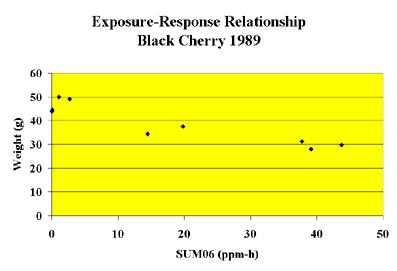
For the tree seedling data, individual Weibull models were fit to each harvest separately. A Weibull regression model was fit to relate tissue biomass with ozone exposure. The figure to the right is an example of yield data obtained in a black cherry experiment performed at Appalachian State University, Boone, NC in 1989. Open-top chambers were used in the experiment. The "y" axis is the yield information (in units of grams) and the "x" axis is the experimental-period SUM06 experienced in each of the chambers. Each data point represents a different ozone level and response as a function of the the treatments used in the experiment.

The basic Weibull yield-response model was used in the A.S.L. & Associates analysis because it was flexible and accommodated a range of data patterns. A Weibull equation of the following form was used:

The three constants, A, B, and C represent (1) the theoretical yield at zero ozone, (2) the scale parameter on ozone exposure and reflects the exposure at which expected response is reduced to 0.37 A, and (3) the shape parameter affecting the change in the rate of loss in expected response, respectively. The x value is the value for the exposure index (e.g., W126 or SUM06) in parts-per-million hours (ppm-h) units.

In the example above, the average weight of the plants in each chamber was used with the SUM06 value experienced in the chamber in fitting the data to a Weibull model. The resulting model provided a way to relate ozone exposure in terms of the SUM06 index with predicted growth loss.

In the analysis performed by A.S.L. & Associates , the Weibull Equations for several vegetation species were used to predict growth loss. However, because the original experimental data derived from the open-top chambers also contained numerous high hourly average concentrations (i.e., equal to and above 0.10 ppm), specific attention was given to these high hourly average concentrations.

Returning to the original experimental data, A.S.L. & Associates examined the number of hourly average concentrations equal to and above 0.10 ppm experienced in each chamber for each experiment. Using this information, A.S.L. & Associates developed separate models that related the number of hourly average concentrations equal to and above 0.10 ppm to the experimental W126 or SUM06 exposure experienced.

In completing the analysis, A.S.L. & Associates combined (a) the information using the Weibull models that predicted growth loss for a specific species in a specific experiment as a function of ozone exposure (e.g., W126) with (b) the predicted number of occurrences equal to and greater than 0.10 ppm. Thus, the predicted species losses were based on a dual-parameter exposure index--

W126

and

Number of hourly average concentrations equal to and greater than 0.10 ppm.

The resulting growth-response curves in the analysis for each species for each year were shown with the growth loss on the "y" axis, the cumulative W126 or SUM06 exposure index on the "x" axis, and the number of occurrences equal to and greater than 0.10 ppm at the 10%, 20%, 30%, etc. growth loss levels that would have to occur. The N100 value at each level of predicted loss was placed on each data point on the curve.

Thus, taking a hypothetical case, if:

The ambient ozone level in a specific area in the region experienced a W126 exposure value of 40 ppm-h and only 1 occurrence of an hourly average concentration equal to and greater than 0.10 ppm

and

Using experimental data, the Weibull model predicted a growth loss of 23% for a specific species grown in the area when the W126 exposure value was 40 ppm-h

and

Using the experimental data, one found that 45 occurrences of hourly average concentrations equal to and greater than 0.10 ppm had to occur at the W126 value of 40 ppm-h.

It is more than likely little growth loss would occur under ambient conditions in the area within the region because of a lack of peak concentrations.

The reason for this prediction is because the ozone exposure under ambient conditions showed infrequent occurrences of the high hourly average concentrations that were present in the original open-top chamber experiments. As noted in the report, EPA emphasized in the Ozone Criteria Document that the higher hourly average concentrations should be treated differently than the mid- and low-level hourly average concentrations. The higher hourly average concentrations should be provided greater weight when assessing possible vegetation effects. Ignoring the presence of the numerous peaks in the open-top chamber experiments essentially treats all hourly average concentrations the same. This is an incorrect application of the findings stated in the Ozone Criteria Document and the conclusions drawn in the peer-review literature.